Notebook Implemented

Baseline language modeling and Code setup¶

Download the dataset from the implementation repository.

In [2]:

#input the dataset and read it in
with open('cleaned_dataset.txt', 'r', encoding='utf-8') as f:
    text = f.read()

#input the dataset and read it in with open('cleaned_dataset.txt', 'r', encoding='utf-8') as f: text = f.read()

In [2]:

print("Length of dataset (in characters): ", len(text))

print("Length of dataset (in characters): ", len(text))

Length of dataset (in characters):  6199345

In [3]:

#The first 1000 characters
print(text[:1000])

#The first 1000 characters print(text[:1000])

M r. and Mrs. Dursley, of number four, Privet Drive, were proud to say that they were perfectly normal, thank you very much. They were the last people youd expect to be involved in anything strange or mysterious, because they just didnt hold with such nonsense.

Mr. Dursley was the director of a firm called Grunnings, which made drills. He was a big, beefy man with hardly any neck, although he did have a very large mustache. Mrs. Dursley was thin and blonde and had nearly twice the usual amount of neck, which came in very useful as she spent so much of her time craning over garden fences, spying on the neighbors. The Dursleys had a small son called Dudley and in their opinion there was no finer boy anywhere.

The Dursleys had everything they wanted, but they also had a secret, and their greatest fear was that somebody would discover it. They didnt think they could bear it if anyone found out about the Potters. Mrs. Potter was Mrs. Dursleys sister, but they hadnt met for several years; 

In [3]:

#Listing all the possible unique characters that occur in our dataset
characters = sorted(list(set(text)))
vocab_size = len(characters)
print(''.join(characters))
print(vocab_size)

#Listing all the possible unique characters that occur in our dataset characters = sorted(list(set(text))) vocab_size = len(characters) print(''.join(characters)) print(vocab_size)

 !"&'()*,-./0123456789:;?ABCDEFGHIJKLMNOPQRSTUVWXYZ[\]^_abcdefghijklmnopqrstuvwxyz{|}
86

Now, we need some strategy to tokenize the input text. When we say tokenize we mean convert the raw text as a string into some sequence of integers according to some vocabulary of possible elements.

 

Here in our case we are going to be building a character level language model - So will be translating individual characters into integers.

 

We will be implementing encoders and decoders, but rather a simple one (as that should be enough for our usecase).

But there are may others (Encoding texts into integers and also decoding them) which use different schema and different vocabularies:

• Google uses sentencepiece: This encoder implements sub-word units. What that means is that it neither considers the entire word nor a single character. And that is what is usually adopted in practice.

• OpenAI uses tiktoken: This uses BPE i.e. Bi Pair Encoding tokenizer and this what GPT uses. Here the vocabulary size is very large, almost upto 50,000 tokens.

So here we have tradeoffs:

• You can have very long sequence integers with a small vocabulary.
• You can have very large vocabulary with a small sequence of integers.

Now, we will be sticking to a character level tokenizer only and we are using a simple encoder and decoder. And our vocabulary size is pretty small i.e. 86 characters (so our tradeoff will be that we will have a large sequence of integers when it is encoded)

In [4]:

# Creating mapping from characters to integers

stoi = { ch:i for i,ch in enumerate(characters) }
itos = { i:ch for i,ch in enumerate(characters) }

encode = lambda s: [stoi[c] for c in s]
decode = lambda l: ''.join([itos[i] for i in l])

#Example to see how the encoding and decoding is happening
# print(encode("harry potter"))
# print(decode(encode("harry potter")))

# Output:
# [64, 57, 74, 74, 81, 1, 72, 71, 76, 76, 61, 74]
# harry potter

# Creating mapping from characters to integers stoi = { ch:i for i,ch in enumerate(characters) } itos = { i:ch for i,ch in enumerate(characters) } encode = lambda s: [stoi[c] for c in s] decode = lambda l: ''.join([itos[i] for i in l]) #Example to see how the encoding and decoding is happening # print(encode("harry potter")) # print(decode(encode("harry potter"))) # Output: # [64, 57, 74, 74, 81, 1, 72, 71, 76, 76, 61, 74] # harry potter

In [5]:

# Now we will be encoding our entire dataset

import torch #I used `pip install torch torchvision torchaudio --index-url https://download.pytorch.org/whl/cu121`my CUDA version is 12.6
data = torch.tensor(encode(text), dtype=torch.long)
print(data.shape , data.size)
print(data[:1000])

# Now we will be encoding our entire dataset import torch #I used `pip install torch torchvision torchaudio --index-url https://download.pytorch.org/whl/cu121`my CUDA version is 12.6 data = torch.tensor(encode(text), dtype=torch.long) print(data.shape , data.size) print(data[:1000])

torch.Size([6199345]) <built-in method size of Tensor object at 0x000002D0CD42BC40>
tensor([38,  1, 74, 11,  1, 57, 70, 60,  1, 38, 74, 75, 11,  1, 29, 77, 74, 75,
        68, 61, 81,  9,  1, 71, 62,  1, 70, 77, 69, 58, 61, 74,  1, 62, 71, 77,
        74,  9,  1, 41, 74, 65, 78, 61, 76,  1, 29, 74, 65, 78, 61,  9,  1, 79,
        61, 74, 61,  1, 72, 74, 71, 77, 60,  1, 76, 71,  1, 75, 57, 81,  1, 76,
        64, 57, 76,  1, 76, 64, 61, 81,  1, 79, 61, 74, 61,  1, 72, 61, 74, 62,
        61, 59, 76, 68, 81,  1, 70, 71, 74, 69, 57, 68,  9,  1, 76, 64, 57, 70,
        67,  1, 81, 71, 77,  1, 78, 61, 74, 81,  1, 69, 77, 59, 64, 11,  1, 45,
        64, 61, 81,  1, 79, 61, 74, 61,  1, 76, 64, 61,  1, 68, 57, 75, 76,  1,
        72, 61, 71, 72, 68, 61,  1, 81, 71, 77, 60,  1, 61, 80, 72, 61, 59, 76,
         1, 76, 71,  1, 58, 61,  1, 65, 70, 78, 71, 68, 78, 61, 60,  1, 65, 70,
         1, 57, 70, 81, 76, 64, 65, 70, 63,  1, 75, 76, 74, 57, 70, 63, 61,  1,
        71, 74,  1, 69, 81, 75, 76, 61, 74, 65, 71, 77, 75,  9,  1, 58, 61, 59,
        57, 77, 75, 61,  1, 76, 64, 61, 81,  1, 66, 77, 75, 76,  1, 60, 65, 60,
        70, 76,  1, 64, 71, 68, 60,  1, 79, 65, 76, 64,  1, 75, 77, 59, 64,  1,
        70, 71, 70, 75, 61, 70, 75, 61, 11,  0,  0, 38, 74, 11,  1, 29, 77, 74,
        75, 68, 61, 81,  1, 79, 57, 75,  1, 76, 64, 61,  1, 60, 65, 74, 61, 59,
        76, 71, 74,  1, 71, 62,  1, 57,  1, 62, 65, 74, 69,  1, 59, 57, 68, 68,
        61, 60,  1, 32, 74, 77, 70, 70, 65, 70, 63, 75,  9,  1, 79, 64, 65, 59,
        64,  1, 69, 57, 60, 61,  1, 60, 74, 65, 68, 68, 75, 11,  1, 33, 61,  1,
        79, 57, 75,  1, 57,  1, 58, 65, 63,  9,  1, 58, 61, 61, 62, 81,  1, 69,
        57, 70,  1, 79, 65, 76, 64,  1, 64, 57, 74, 60, 68, 81,  1, 57, 70, 81,
         1, 70, 61, 59, 67,  9,  1, 57, 68, 76, 64, 71, 77, 63, 64,  1, 64, 61,
         1, 60, 65, 60,  1, 64, 57, 78, 61,  1, 57,  1, 78, 61, 74, 81,  1, 68,
        57, 74, 63, 61,  1, 69, 77, 75, 76, 57, 59, 64, 61, 11,  1, 38, 74, 75,
        11,  1, 29, 77, 74, 75, 68, 61, 81,  1, 79, 57, 75,  1, 76, 64, 65, 70,
         1, 57, 70, 60,  1, 58, 68, 71, 70, 60, 61,  1, 57, 70, 60,  1, 64, 57,
        60,  1, 70, 61, 57, 74, 68, 81,  1, 76, 79, 65, 59, 61,  1, 76, 64, 61,
         1, 77, 75, 77, 57, 68,  1, 57, 69, 71, 77, 70, 76,  1, 71, 62,  1, 70,
        61, 59, 67,  9,  1, 79, 64, 65, 59, 64,  1, 59, 57, 69, 61,  1, 65, 70,
         1, 78, 61, 74, 81,  1, 77, 75, 61, 62, 77, 68,  1, 57, 75,  1, 75, 64,
        61,  1, 75, 72, 61, 70, 76,  1, 75, 71,  1, 69, 77, 59, 64,  1, 71, 62,
         1, 64, 61, 74,  1, 76, 65, 69, 61,  1, 59, 74, 57, 70, 65, 70, 63,  1,
        71, 78, 61, 74,  1, 63, 57, 74, 60, 61, 70,  1, 62, 61, 70, 59, 61, 75,
         9,  1, 75, 72, 81, 65, 70, 63,  1, 71, 70,  1, 76, 64, 61,  1, 70, 61,
        65, 63, 64, 58, 71, 74, 75, 11,  1, 45, 64, 61,  1, 29, 77, 74, 75, 68,
        61, 81, 75,  1, 64, 57, 60,  1, 57,  1, 75, 69, 57, 68, 68,  1, 75, 71,
        70,  1, 59, 57, 68, 68, 61, 60,  1, 29, 77, 60, 68, 61, 81,  1, 57, 70,
        60,  1, 65, 70,  1, 76, 64, 61, 65, 74,  1, 71, 72, 65, 70, 65, 71, 70,
         1, 76, 64, 61, 74, 61,  1, 79, 57, 75,  1, 70, 71,  1, 62, 65, 70, 61,
        74,  1, 58, 71, 81,  1, 57, 70, 81, 79, 64, 61, 74, 61, 11,  0,  0, 45,
        64, 61,  1, 29, 77, 74, 75, 68, 61, 81, 75,  1, 64, 57, 60,  1, 61, 78,
        61, 74, 81, 76, 64, 65, 70, 63,  1, 76, 64, 61, 81,  1, 79, 57, 70, 76,
        61, 60,  9,  1, 58, 77, 76,  1, 76, 64, 61, 81,  1, 57, 68, 75, 71,  1,
        64, 57, 60,  1, 57,  1, 75, 61, 59, 74, 61, 76,  9,  1, 57, 70, 60,  1,
        76, 64, 61, 65, 74,  1, 63, 74, 61, 57, 76, 61, 75, 76,  1, 62, 61, 57,
        74,  1, 79, 57, 75,  1, 76, 64, 57, 76,  1, 75, 71, 69, 61, 58, 71, 60,
        81,  1, 79, 71, 77, 68, 60,  1, 60, 65, 75, 59, 71, 78, 61, 74,  1, 65,
        76, 11,  1, 45, 64, 61, 81,  1, 60, 65, 60, 70, 76,  1, 76, 64, 65, 70,
        67,  1, 76, 64, 61, 81,  1, 59, 71, 77, 68, 60,  1, 58, 61, 57, 74,  1,
        65, 76,  1, 65, 62,  1, 57, 70, 81, 71, 70, 61,  1, 62, 71, 77, 70, 60,
         1, 71, 77, 76,  1, 57, 58, 71, 77, 76,  1, 76, 64, 61,  1, 41, 71, 76,
        76, 61, 74, 75, 11,  1, 38, 74, 75, 11,  1, 41, 71, 76, 76, 61, 74,  1,
        79, 57, 75,  1, 38, 74, 75, 11,  1, 29, 77, 74, 75, 68, 61, 81, 75,  1,
        75, 65, 75, 76, 61, 74,  9,  1, 58, 77, 76,  1, 76, 64, 61, 81,  1, 64,
        57, 60, 70, 76,  1, 69, 61, 76,  1, 62, 71, 74,  1, 75, 61, 78, 61, 74,
        57, 68,  1, 81, 61, 57, 74, 75, 24,  1])

Now we get to the interesting part (atleast for me lol), we will be splitting the train and validation set. In our case we will be taking 90% for training and remaining for validation. The reason is we dont want our model to completely memorise the dataset and instead generate 'Harry Potter' like texts, hence we are witholding some information and will be using it to check for overfitting at the end.

In [6]:

n = int(0.9*len(data))
train_data = data[:n]
val_data = data[n:]

n = int(0.9*len(data)) train_data = data[:n] val_data = data[n:]

Okay so now, we never feed our entire data into the model, as that would be computationally expensive and prohibitive. So we divide them into blocks and then group all those blocks into batches and then train them. Each batch is independently trainied and are not communicating with each other.

In [7]:

torch.manual_seed(3007) # My dataset is different from what sensei is using, so i am using my own random number here :)
batch_size = 4 # how many independent sequences will we process in parallel?
block_size = 8 # what is the maximum context length for predictions?

def get_batch(split):
    # generate a small batch of data of inputs x and targets y
    data = train_data if split == 'train' else val_data #if the function call is for train then it considers train data else the val data
    ix = torch.randint(len(data) - block_size, (batch_size,)) #this one takes the random chunk of values
    x = torch.stack([data[i:i+block_size] for i in ix]) #x is the first array which will take the values
    y = torch.stack([data[i+1:i+block_size+1] for i in ix]) #y is the second array which will consider the respective target values ("the next character that needs to be predicted")
    return x, y

xb, yb = get_batch('train')
print('inputs:')
print(xb.shape)
print(xb)
print('targets:')
print(yb.shape)
print(yb)

print('----')

for b in range(batch_size): # batch dimension
    for t in range(block_size): # time dimension
        context = xb[b, :t+1]
        target = yb[b,t]
        print(f"when input is {context.tolist()} the target: {target}")

torch.manual_seed(3007) # My dataset is different from what sensei is using, so i am using my own random number here :) batch_size = 4 # how many independent sequences will we process in parallel? block_size = 8 # what is the maximum context length for predictions? def get_batch(split): # generate a small batch of data of inputs x and targets y data = train_data if split == 'train' else val_data #if the function call is for train then it considers train data else the val data ix = torch.randint(len(data) - block_size, (batch_size,)) #this one takes the random chunk of values x = torch.stack([data[i:i+block_size] for i in ix]) #x is the first array which will take the values y = torch.stack([data[i+1:i+block_size+1] for i in ix]) #y is the second array which will consider the respective target values ("the next character that needs to be predicted") return x, y xb, yb = get_batch('train') print('inputs:') print(xb.shape) print(xb) print('targets:') print(yb.shape) print(yb) print('----') for b in range(batch_size): # batch dimension for t in range(block_size): # time dimension context = xb[b, :t+1] target = yb[b,t] print(f"when input is {context.tolist()} the target: {target}")

inputs:
torch.Size([4, 8])
tensor([[79, 57, 68, 67, 65, 70, 63,  1],
        [64,  1, 57, 70, 63, 74, 81,  1],
        [ 1, 69, 65, 60, 57, 65, 74,  9],
        [ 1, 60, 65, 60,  1, 65, 76,  1]])
targets:
torch.Size([4, 8])
tensor([[57, 68, 67, 65, 70, 63,  1, 57],
        [ 1, 57, 70, 63, 74, 81,  1, 57],
        [69, 65, 60, 57, 65, 74,  9,  1],
        [60, 65, 60,  1, 65, 76,  1, 65]])
----
when input is [79] the target: 57
when input is [79, 57] the target: 68
when input is [79, 57, 68] the target: 67
when input is [79, 57, 68, 67] the target: 65
when input is [79, 57, 68, 67, 65] the target: 70
when input is [79, 57, 68, 67, 65, 70] the target: 63
when input is [79, 57, 68, 67, 65, 70, 63] the target: 1
when input is [79, 57, 68, 67, 65, 70, 63, 1] the target: 57
when input is [64] the target: 1
when input is [64, 1] the target: 57
when input is [64, 1, 57] the target: 70
when input is [64, 1, 57, 70] the target: 63
when input is [64, 1, 57, 70, 63] the target: 74
when input is [64, 1, 57, 70, 63, 74] the target: 81
when input is [64, 1, 57, 70, 63, 74, 81] the target: 1
when input is [64, 1, 57, 70, 63, 74, 81, 1] the target: 57
when input is [1] the target: 69
when input is [1, 69] the target: 65
when input is [1, 69, 65] the target: 60
when input is [1, 69, 65, 60] the target: 57
when input is [1, 69, 65, 60, 57] the target: 65
when input is [1, 69, 65, 60, 57, 65] the target: 74
when input is [1, 69, 65, 60, 57, 65, 74] the target: 9
when input is [1, 69, 65, 60, 57, 65, 74, 9] the target: 1
when input is [1] the target: 60
when input is [1, 60] the target: 65
when input is [1, 60, 65] the target: 60
when input is [1, 60, 65, 60] the target: 1
when input is [1, 60, 65, 60, 1] the target: 65
when input is [1, 60, 65, 60, 1, 65] the target: 76
when input is [1, 60, 65, 60, 1, 65, 76] the target: 1
when input is [1, 60, 65, 60, 1, 65, 76, 1] the target: 65

The explaination for above is rather simple, in the first array we have the batch of data which we have considered and each row is the block of data. The second array shows us what the target value will be for the corresponding value in the first array.

For example, In first array value is 79 -> so in target array its value will be 57 In first array value is 79, 57 -> so in target array its value will be 68 and so on

In [8]:

print(xb)

print(xb)

tensor([[79, 57, 68, 67, 65, 70, 63,  1],
        [64,  1, 57, 70, 63, 74, 81,  1],
        [ 1, 69, 65, 60, 57, 65, 74,  9],
        [ 1, 60, 65, 60,  1, 65, 76,  1]])

Since we now have our first set of data which we need to feed into our transformer, we will now implement the simplest model - therefore, the bigram languuage model in pytorch.

 

Okay so the lecture goes on from the 22nd minute to the 34th, there was a lot of quick breakdown of the code since it was already done in the previous videos (i still couldn't get some of the visuals as to why we did what we did, but lets see how this goes). Also right now, the output maybe a little silly, but apparently we will be needing this generate function in the bigram model class later in the end when we want the model to refer the history of the sentences formed (like if we are at one point in a sentence, then need it to keep track of the previous characters generated up until that point).

In [2]:

import torch
import torch.nn as nn
from torch.nn import functional as F

import torch import torch.nn as nn from torch.nn import functional as F

In [ ]:

torch.manual_seed(3007)

class BigramLanguageModel(nn.Module):

    def __init__(self, vocab_size):
        super().__init__()
        # each token directly reads off the logits for the next token from a lookup table
        self.token_embedding_table = nn.Embedding(vocab_size, vocab_size)

    def forward(self, idx, targets=None):

        # idx and targets are both (B,T) tensor of integers
        logits = self.token_embedding_table(idx) # (B,T,C)

        if targets is None:
            loss = None
        else:
            B, T, C = logits.shape
            logits = logits.view(B*T, C)
            targets = targets.view(B*T)
            loss = F.cross_entropy(logits, targets)

        return logits, loss

    def generate(self, idx, max_new_tokens):
        # idx is (B, T) array of indices in the current context
        for _ in range(max_new_tokens):
            # get the predictions
            logits, loss = self(idx)
            # focus only on the last time step
            logits = logits[:, -1, :] # becomes (B, C)
            # apply softmax to get probabilities
            probs = F.softmax(logits, dim=-1) # (B, C)
            # sample from the distribution
            idx_next = torch.multinomial(probs, num_samples=1) # (B, 1)
            # append sampled index to the running sequence
            idx = torch.cat((idx, idx_next), dim=1) # (B, T+1)
        return idx

m = BigramLanguageModel(vocab_size)
logits, loss = m(xb, yb)
print(logits.shape)
print(loss)

print(decode(m.generate(idx = torch.zeros((1, 1), dtype=torch.long), max_new_tokens=100)[0].tolist()))

torch.manual_seed(3007) class BigramLanguageModel(nn.Module): def __init__(self, vocab_size): super().__init__() # each token directly reads off the logits for the next token from a lookup table self.token_embedding_table = nn.Embedding(vocab_size, vocab_size) def forward(self, idx, targets=None): # idx and targets are both (B,T) tensor of integers logits = self.token_embedding_table(idx) # (B,T,C) if targets is None: loss = None else: B, T, C = logits.shape logits = logits.view(B*T, C) targets = targets.view(B*T) loss = F.cross_entropy(logits, targets) return logits, loss def generate(self, idx, max_new_tokens): # idx is (B, T) array of indices in the current context for _ in range(max_new_tokens): # get the predictions logits, loss = self(idx) # focus only on the last time step logits = logits[:, -1, :] # becomes (B, C) # apply softmax to get probabilities probs = F.softmax(logits, dim=-1) # (B, C) # sample from the distribution idx_next = torch.multinomial(probs, num_samples=1) # (B, 1) # append sampled index to the running sequence idx = torch.cat((idx, idx_next), dim=1) # (B, T+1) return idx m = BigramLanguageModel(vocab_size) logits, loss = m(xb, yb) print(logits.shape) print(loss) print(decode(m.generate(idx = torch.zeros((1, 1), dtype=torch.long), max_new_tokens=100)[0].tolist()))

torch.Size([32, 86])
tensor(4.9531, grad_fn=<NllLossBackward0>)

1fzM0Fy_Bufz 1/cPH9mF_c/CYk]kZ573w8,2 \Oww)(y&9D9,HzR]
MOpFbp[&vdr[D9QO4Kl)qKhWCuifZ3YXyi[IK"\-8IZdD

Okay so now, we are going to train this above model, we will first declare an optimizer called AdamW which is a lot more advance than the one we have been using previously which was the gradient descent optimizer which can also be invoked using SGD but that is the simplest one so we are not going ahead with that.

 

So at the end of this we are expecting a slightly, very slightly improvements of the output from the above cell (obviously can't expect much because this is a bigram model)

In [11]:

# create a PyTorch optimizer
optimizer = torch.optim.AdamW(m.parameters(), lr=1e-3)

# create a PyTorch optimizer optimizer = torch.optim.AdamW(m.parameters(), lr=1e-3)

In [15]:

#Play around with the range value, increase it and see the loss improves overtime, once you see a small enough value (atleast maybe 2.5), stop and check your output in the next cell!

batch_size = 32
for steps in range(10000): # increase number of steps for good results...

    # sample a batch of data
    xb, yb = get_batch('train')

    # evaluate the loss
    logits, loss = m(xb, yb)
    optimizer.zero_grad(set_to_none=True)
    loss.backward()
    optimizer.step()

print(loss.item())

#Play around with the range value, increase it and see the loss improves overtime, once you see a small enough value (atleast maybe 2.5), stop and check your output in the next cell! batch_size = 32 for steps in range(10000): # increase number of steps for good results... # sample a batch of data xb, yb = get_batch('train') # evaluate the loss logits, loss = m(xb, yb) optimizer.zero_grad(set_to_none=True) loss.backward() optimizer.step() print(loss.item())

2.438239336013794

In [17]:

print(decode(m.generate(idx = torch.zeros((1, 1), dtype=torch.long), max_new_tokens=500)[0].tolist()))

print(decode(m.generate(idx = torch.zeros((1, 1), dtype=torch.long), max_new_tokens=500)[0].tolist()))

Th hatI UI, Er oprr wadiomacalse he ffoinele he entich are Nond t eng pasig n the Rokisthe fouthay ry nld Hahabetond IDemeckny yild:Pryo the FIngl, wasioo whed whed id ht crok the r. ofthe stham, whted r monalimind . ll tt menteacile avit be the wand t I Anditan deeveysseishaintained wad hery, g t th cl bres ditiver, herithethened?' nithe NJferrdeng to Du-ce pe t h, awhemin1|jousis. teaby Us. t p e sprusw in ag tt t caunong on, he y It way r herd wa as.

' iqutshotadng  hitrstwe che s As Ha

Eh, not bad (jk its gibberish, but hey its forming words in a sentence format yay hahah)

Okay so better explaination on whats happening above:

What we are doing here is that, the tokens are not really talking to each other.

Here, although we are passing the entire previous characters, we are only considering the last charcter in that sequence to predict the next one (so now you see why this is a very simple model. So in the above output sentence Th hatI UI, Er, for predicting r it only considered E from the entire sequence of previous characters). We can see that in the code section logits = logits[:, -1, :] where -1 is added.

Next what we want to do is that we want the tokens to communicate with each other so that there is more context to what needs to be generated next. Therefore allowing us to move into transformers.

 

Note: Added a bigram.py file which is essentially a python script containing all of the above implemented code. You can run it and see the output produced (There are some modifications to it, where if you have CUDA it utilises it and moves the training inputs, models to it etc. Along with knowing which mode your model is in- whether it is train or val. Apparently this isnt that important for a bigram model, but it is good practise)

---

Building the "self-attention"¶

From minute 42nd to 58th, sensei explains the mathematical trick to self-attention and he uses three versions to explain it. Essentially it is matrix multiplication of the lower triangle of the matrix.

To summarise it more clearly:

• You can do weighted aggregations of your past elements, by using matrix multiplications of a lower triangular fashion.
• And the elements in the lower triangular part, are telling you how much each element fuses into the final position. Therefore, we are using this to develop the self attention block.

This is what that matrix would look like:

1 0 0 0 0
1 1 0 0 0
1 1 1 0 0
1 1 1 1 0
1 1 1 1 1

Self-Attention breakdown implementation

In [3]:

# version 4: self-attention!
torch.manual_seed(1337)
B,T,C = 4,8,32 # batch, time, channels
x = torch.randn(B,T,C)

# let's see a single Head perform self-attention
head_size = 16
key = nn.Linear(C, head_size, bias=False)
query = nn.Linear(C, head_size, bias=False)
value = nn.Linear(C, head_size, bias=False)
k = key(x)   # (B, T, 16)
q = query(x) # (B, T, 16)
wei =  q @ k.transpose(-2, -1) # (B, T, 16) @ (B, 16, T) ---> (B, T, T)

tril = torch.tril(torch.ones(T, T))
#wei = torch.zeros((T,T))
wei = wei.masked_fill(tril == 0, float('-inf'))
wei = F.softmax(wei, dim=-1)

v = value(x)
out = wei @ v
#out = wei @ x

out.shape

# version 4: self-attention! torch.manual_seed(1337) B,T,C = 4,8,32 # batch, time, channels x = torch.randn(B,T,C) # let's see a single Head perform self-attention head_size = 16 key = nn.Linear(C, head_size, bias=False) query = nn.Linear(C, head_size, bias=False) value = nn.Linear(C, head_size, bias=False) k = key(x) # (B, T, 16) q = query(x) # (B, T, 16) wei = q @ k.transpose(-2, -1) # (B, T, 16) @ (B, 16, T) ---> (B, T, T) tril = torch.tril(torch.ones(T, T)) #wei = torch.zeros((T,T)) wei = wei.masked_fill(tril == 0, float('-inf')) wei = F.softmax(wei, dim=-1) v = value(x) out = wei @ v #out = wei @ x out.shape

Out[3]:

torch.Size([4, 8, 16])

In [4]:

wei[0]

wei[0]

Out[4]:

tensor([[1.0000, 0.0000, 0.0000, 0.0000, 0.0000, 0.0000, 0.0000, 0.0000],
        [0.1574, 0.8426, 0.0000, 0.0000, 0.0000, 0.0000, 0.0000, 0.0000],
        [0.2088, 0.1646, 0.6266, 0.0000, 0.0000, 0.0000, 0.0000, 0.0000],
        [0.5792, 0.1187, 0.1889, 0.1131, 0.0000, 0.0000, 0.0000, 0.0000],
        [0.0294, 0.1052, 0.0469, 0.0276, 0.7909, 0.0000, 0.0000, 0.0000],
        [0.0176, 0.2689, 0.0215, 0.0089, 0.6812, 0.0019, 0.0000, 0.0000],
        [0.1691, 0.4066, 0.0438, 0.0416, 0.1048, 0.2012, 0.0329, 0.0000],
        [0.0210, 0.0843, 0.0555, 0.2297, 0.0573, 0.0709, 0.2423, 0.2391]],
       grad_fn=<SelectBackward0>)

Notes:

• Attention is a communication mechanism. Can be seen as nodes in a directed graph looking at each other and aggregating information with a weighted sum from all nodes that point to them, with data-dependent weights.
• There is no notion of space. Attention simply acts over a set of vectors. This is why we need to positionally encode tokens.
• Each example across batch dimension is of course processed completely independently and never "talk" to each other
• In an "encoder" attention block just delete the single line that does masking with tril, allowing all tokens to communicate. This block here is called a "decoder" attention block because it has triangular masking, and is usually used in autoregressive settings, like language modeling.
• "self-attention" just means that the keys and values are produced from the same source as queries. In "cross-attention", the queries still get produced from x, but the keys and values come from some other, external source (e.g. an encoder module)
• "Scaled" attention additional divides wei by 1/sqrt(head_size). This makes it so when input Q,K are unit variance, wei will be unit variance too and Softmax will stay diffuse and not saturate too much. Illustration below

---

Building the Transformer¶

Implementation of the Tranformer model diagram.

 

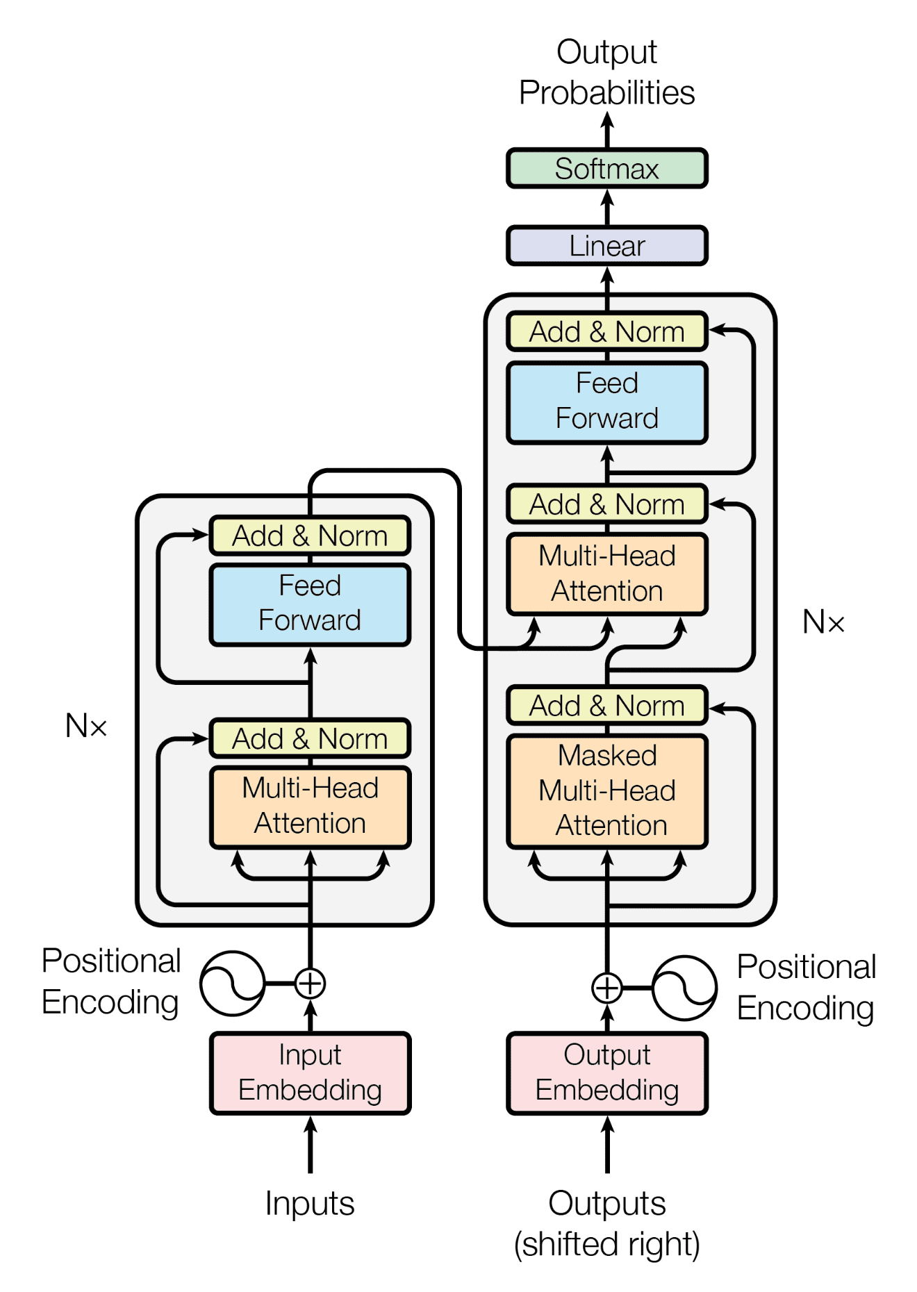
(⚠️Note: Do not run the following cells, I have split them up for explaination breakdown purposes. You can find the final script here in gpt.py)

 

Inserting a Single Self Attention block: Here we have implemented a module called 'Head' which is a single head implementation of self attention.

In [ ]:

class Head(nn.Module)

class Head(nn.Module)

In [ ]:

def __init__(self, head_size):
    super().__init__()
    self.key = nn.Linear(n_embd, head_size, bias=False)
    self.query = nn.Linear(n_embd, head_size, bias=False)
    self.value = nn.Linear(n_embd, head_size, bias=False)
    self.register_buffer('tril', torch.tril(torch.ones(block_size, block_size)))

    self.dropout = nn.Dropout(dropout)

def __init__(self, head_size): super().__init__() self.key = nn.Linear(n_embd, head_size, bias=False) self.query = nn.Linear(n_embd, head_size, bias=False) self.value = nn.Linear(n_embd, head_size, bias=False) self.register_buffer('tril', torch.tril(torch.ones(block_size, block_size))) self.dropout = nn.Dropout(dropout)

• We are giving the input head_size and we are passing it to the key, query and value - Linear layers. People don't usually use bias for these so they are set to false.
• tril is not a parameter (this is what makes that lower triangle in the matrix example that we saw), so considering the "PyTorch naming convintion" we register them as buffers so that we can assign it to the module.

In [ ]:

def forward(self, x):
       # input of size (batch, time-step, channels)
       # output of size (batch, time-step, head size)
       B,T,C = x.shape
       k = self.key(x)   # (B,T,hs)
       q = self.query(x) # (B,T,hs)
       # compute attention scores ("affinities")
       wei = q @ k.transpose(-2,-1) * k.shape[-1]**-0.5 # (B, T, hs) @ (B, hs, T) -> (B, T, T)
       wei = wei.masked_fill(self.tril[:T, :T] == 0, float('-inf')) # (B, T, T)
       wei = F.softmax(wei, dim=-1) # (B, T, T)
       wei = self.dropout(wei)
       # perform the weighted aggregation of the values
       v = self.value(x) # (B,T,hs)
       out = wei @ v # (B, T, T) @ (B, T, hs) -> (B, T, hs)
       return out

def forward(self, x): # input of size (batch, time-step, channels) # output of size (batch, time-step, head size) B,T,C = x.shape k = self.key(x) # (B,T,hs) q = self.query(x) # (B,T,hs) # compute attention scores ("affinities") wei = q @ k.transpose(-2,-1) * k.shape[-1]**-0.5 # (B, T, hs) @ (B, hs, T) -> (B, T, T) wei = wei.masked_fill(self.tril[:T, :T] == 0, float('-inf')) # (B, T, T) wei = F.softmax(wei, dim=-1) # (B, T, T) wei = self.dropout(wei) # perform the weighted aggregation of the values v = self.value(x) # (B,T,hs) out = wei @ v # (B, T, T) @ (B, T, hs) -> (B, T, hs) return out

• We passing x as the input, calculating the key and query.
• Then we are calculating the attention scores inside wei.
• Here we are making sure that tril doesn't communicate with the future (the additional values beyond the character point we are in) wei = wei.masked_fill(self.tril[:T, :T] == 0, float('-inf')) so that acts as a decoder block.
• Then its the softmax, aggregating the value and out.

 

Implementing the Multi-Head Attention Layer

In [ ]:

class MultiHeadAttention(nn.Module):

    def __init__(self, num_heads, head_size):
        super().__init__()
        self.heads = nn.ModuleList([Head(head_size) for _ in range(num_heads)])
        self.proj = nn.Linear(head_size * num_heads, n_embd)
        self.dropout = nn.Dropout(dropout)

    def forward(self, x):
        out = torch.cat([h(x) for h in self.heads], dim=-1)
        out = self.dropout(self.proj(out))
        return out

class MultiHeadAttention(nn.Module): def __init__(self, num_heads, head_size): super().__init__() self.heads = nn.ModuleList([Head(head_size) for _ in range(num_heads)]) self.proj = nn.Linear(head_size * num_heads, n_embd) self.dropout = nn.Dropout(dropout) def forward(self, x): out = torch.cat([h(x) for h in self.heads], dim=-1) out = self.dropout(self.proj(out)) return out

• Here we want multiple heads of self attention running in parallel. So in pytorch you mention the number of heads and the head size, and you run all of them in parallel into a list. Finally, you simply just concatenate all of the outputs and we are concatenating over the channel dimension (dim=-1)
• So this allows the tokens to communicate with each other, like the vowels, the correlation between them and finding different things, so this helps in providing different communication channels allowing the gathering of different types of data and decode the output.

 

Implementing Feed Forward

In [ ]:

class FeedFoward(nn.Module):

    def __init__(self, n_embd):
        super().__init__()
        self.net = nn.Sequential(
            nn.Linear(n_embd, 4 * n_embd),
            nn.ReLU(),
            nn.Linear(4 * n_embd, n_embd),
            nn.Dropout(dropout),
        )

    def forward(self, x):
        return self.net(x)

class FeedFoward(nn.Module): def __init__(self, n_embd): super().__init__() self.net = nn.Sequential( nn.Linear(n_embd, 4 * n_embd), nn.ReLU(), nn.Linear(4 * n_embd, n_embd), nn.Dropout(dropout), ) def forward(self, x): return self.net(x)

• After the self attention where the tokens are communicating with each other, they need to start processing it individually to understand and that is where feed forwarding comes in. So Linear layer is applied on a per token level.
• So you can say that after the 'communication' in the previous layer, here is where the model 'computes' them.
• The 4 * is done because in the paper for that layer they have mentioned that for them the dimensionality of input and output is 512 and the inner layer is 2048, basically the inner layer is 4 times the value, therefore we've added that as well. And the parameters are switched i.e. (n_embd, 4 * n_embd) then nn.Linear(4 * n_embd, n_embd) for the implementation of residual connections.  

Putting both the communication and computational modules together in a Block

In [ ]:

class Block(nn.Module):

    def __init__(self, n_embd, n_head):
        # n_embd: embedding dimension, n_head: the number of heads we'd like
        super().__init__()
        head_size = n_embd // n_head
        self.sa = MultiHeadAttention(n_head, head_size)
        self.ffwd = FeedFoward(n_embd)
        self.ln1 = nn.LayerNorm(n_embd)
        self.ln2 = nn.LayerNorm(n_embd)

class Block(nn.Module): def __init__(self, n_embd, n_head): # n_embd: embedding dimension, n_head: the number of heads we'd like super().__init__() head_size = n_embd // n_head self.sa = MultiHeadAttention(n_head, head_size) self.ffwd = FeedFoward(n_embd) self.ln1 = nn.LayerNorm(n_embd) self.ln2 = nn.LayerNorm(n_embd)

• Overall that is what is happening in the transformer model diagram as well, all the self attention layer communication (except one where cross attention is happening, we haven't implemented that in this) and then the feed forwarding computation are grouped together in a Block which is represented as Nx in the diagram.
• Therefore we have the Block module where we have the communications taking place in MultiHeadAttention(n_head, head_size) followed by the computation FeedFoward(n_embd).

In [ ]:

def forward(self, x):
        x = x + self.sa(self.ln1(x))
        x = x + self.ffwd(self.ln2(x))
        return x

def forward(self, x): x = x + self.sa(self.ln1(x)) x = x + self.ffwd(self.ln2(x)) return x

• Residual connection is implemented here x = x + <self attention and feed forward layer calls>

 

• This is the Add part in the transformer model diagram within Add & Norm.
• The Norm in that is basically a Layer Norm, and for that implementation we just do our Batch Normalisation (obviously cutting out some of the parts for example the buffers which were not required).
• Turns out, in the current implementation of Transformer model, there are very few changes to it but we now implement the 'Add & Norm' layer before the Multi Head Self attention block (and that is what we have implemented). This is what we see in self.ln1 = nn.LayerNorm(n_embd), self.ln2 = nn.LayerNorm(n_embd).

 

Finally, Scaling up the model

There were some final touch ups done to the code including:

• n_layer, n_head (in GPTLanguageModel class)
• Adding a nn.Dropout(dropout) (see feed forward, multi head and head classes), which was taken from this paper, see diagram in page 2, where it just freezes some of the nodes during both the forward and backward pass basically and we are using this as a regularization technique as we are scaling up the model (and concerned about overfitting).
• Hyperparameter values have also been changed.

 

• The final complete code can be found here
• The output produced can be viewed here.

 

Final Thoughts: You will notice that the output won't be too great, as this is a transformer model trained on a character level, based on just the 6 million characters dataset on Harry Potter novels. Lastly, this is a decoder only transformer model as we see on GPT, So it only generates texts similar to what was fed into it. The additional layer of self attention, cross attention and decoder block haven't been implemented as they served a different purpose while the paper was written (it was written for you can say language translation, as the encoding was to convert from one language to another. The translated language is what we would have seen from the decoder).

---