Section 1 - B
Sample, auto-detect the device
At the end of the previous section, we had loaded the pretrained gpt2 model and its weights into our architecture and generated the model. But now we could like to initialize our own weights, we want the model to weights to be generated randomly.
So that can be done fairly simple way:
#model = GPT.from_pretrained("gpt2")
model = GPT(GPTConfig())
we just call our default GPTConfig() that we made. So what PyTorch does is that, it internally assigns random weights to each of the layers in our config, therefore we can use this to generate text from our model.
Lastly, before i run this, we also added an additional line of code to better control the device used to run this model. In my case i do have a GPU with CUDA capability. So, if you want to run the model until this point you can also do that using CPU. We have added this additional flag point just to show which device you are using here:
device = "cpu"
if torch.cuda.is_available():
    device = "cuda"

print(f"Device used: {device})
The rest of the code follows a dynamic approach of detecting the device as well (even in the forward() you will see that we have used device=idx.device), therefore we are ensuring that all the layers are using the same device while generating.
And this is the final output that we generated!
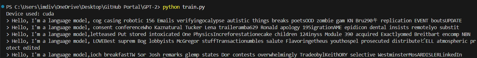
Obviously it is gibberish lol, we will get to the training next!
Let’s train: data batches (B,T) → logits (B,T,C)
NOTE
We will be loading our dataset now. Sensei used his fav "The tiny Shakespear dataset", I am going ahead and using MY Favourite dataset which is what i also used for my GPT-1 implementation which is the HARRY POTTER NOVELS COLLECTION dataset. I directly took the
cleaned_dataset.txtfile which i had processed.If you want to see a simple breakdown version of the dataset and what we are about to do, take a look at this notebook on my repo.
device = "cpu"
if torch.cuda.is_available():
    device = "cuda"

print(f"Device used: {device}")

num_return_sequences = 5
max_length = 30

#==========THIS SECTION==========
import tiktoken
enc = tiktoken.get_encoding('gpt2')

with open('cleaned_dataset.txt', 'r') as f:
    text = f.read()

data = text[:1000]
tokens = enc.encode(data)

B, T = 4, 32
buf = torch.tensor(tokens[:B*T + 1])
x = buf[:-1].view(B, T)
y = buf[1:].view(B, T)
#================================

#model = GPT.from_pretrained("gpt2")
model = GPT(GPTConfig())
model.eval()
model.to(device)

#==========THIS SECTION==========
x = x.to(device)
logits = model(x)
print(logits.shape)
import sys; sys.exit(0)
#================================
So the above SECTIONS are the newly added codes just like how they were done in the dataset breakdown notebook, we are only performing a debugging step here therefore the values have been hardcoded. Since we have a batch of 4 by 32, we get the logits for that.
The output we got when the program was run (notice there is a sys exit):
torch.Size([4, 32, 50257])So
50257are the logits for what comes next at every position. That is thex.
Debugging moment, yay! (Mini version)
So, i had encountered the error RuntimeError: Expected all tensors to be on the same device, but found at least two devices, cuda:0 and cpu!.
This wouldn't happen in sensei's video as he had a manual OVERIDE of the device to cpu. In my case i am continuing to stick with cuda. But since our buffer was initialised manually here: buf = torch.tensor(tokens[:B*T + 1]), it by default sits in the cpu.
To fix this, we just added one additional line of code: x = x.to(device) just before calculating the logits.
Next we still have the y which contains the targets. So now is the time to calculate the loss -> do the backward pass -> and do the optimization. Lets go ahead and calculate the loss first.
Cross entropy loss
#====================
x = x.to(device)
y = y.to(device)    #newly added

# logits = model(x)
logits, loss = model(x, y)  #newly added

# print(logits.shape)
print(loss)     #newly added

import sys; sys.exit(0)
#====================
def forward(self, idx, targets=None): #newly modified

        B, T = idx.size()

        assert T <= self.config.block_size, f"Cannot forward this sequence which is of length {T} as the block size is only {self.config.block_size}"

        pos = torch.arange(0, T, dtype=torch.long, device=idx.device)
        pos_emd = self.transformer.wpe(pos)
        tok_emb = self.transformer.wte(idx)
        x = tok_emb + pos_emd

        for block in self.transformer.h:
            x = block(x)

        x = self.transformer.ln_f(x)

        logits = self.lm_head(x)

        loss = None                     #newly added
        if targets is not None:         #newly added
            loss = F.cross_entropy(logits.view(-1, logits.size(-1)), targets.view(-1))      #newly added

        return logits, loss             #newly modified
In the above code snippets, we are calculating the loss and we will do that by modifing the forward() function by passing an additional (optional) parameter.
So in the function call we do logits, loss = model(x, y) and finally in the function we add the new optional parameter def forward(self, idx, targets=None).
Then if targets are present (which in our case right now, we do) then we need to calculate the loss and we are using the cross_entropy function from PyTorch. So two things are happening here:
- cross_entropy can't take multi-dimensional inputs, so in our case, first we have the logits which is in shape (B, T, vocab_size), so we are flattening that out to two-dimension.
- Is the targets, which is in two-dimensional while passing into the function (as we only made it that way), and while calculating the loss that is turned into one-dimension tensors by the cross_entropy function.
Finally, we get the loss and return the value. (Note: The same mini debugging moment had to be done for y as well.) The output we got is:
Device used: cuda
tensor(10.9997, device='cuda:0', grad_fn=<NllLossBackward0>)
(IMPORTANT POINTS- Callback to previous videos)
The above
lossvalue is actually significant. That is basically the value of a single tensor in our vocabulary.In the previous videos, we have seen that while initialising networks with random values, we needed to ensure that we get a good starting point. And that is achieved by ensuring that the probabilties of the tokens i.e. the values of the individual tensors are almost uniformly distributed, this way we are not favouring any tokens specifically during initialization.
So, in our case, we know that our vocab size is 50257. To calculate the even probability for every token we do:
1 / 50257and then we do the loss calculation. Remember that cross_entropy essentially does negative log likelihood, so when we do that-ln(1/50257)we get a value ~10.8 which is actually the loss value we EXPECT at initialization for the respective model.Therefore, ours being 10.9 shows us that we are at a good starting point and our probabilty distribution is roughly diffused.
So at this point we can do a loss.backward(), calculate the gradients and then do an optimization!
Optimization loop: overfit a single batch
optimizer = torch.optim.AdamW(model.parameters(), lr=3e-4)
for i in range(50):
    optimizer.zero_grad()
    logits, loss = model(x, y)
    loss.backward()
    optimizer.step()
    print(f"Step {i} -> loss value: {loss.item()}")
Okay so here we are doing optimization on a small set of batch and trying to overfit them. Just as a short term example.
We first declare the optimizer object using pytorch and we use the
AdamWoptimizer. We used to use Stochastic Gradient one and then Adam is also used, but it seemsAdamWis a bug fix version of Adam, so we are going ahead with that. We don't really have to know its workings to the depth, for now we will treat this as a black box itself. Ultimately, its aim is to speed up this whole optimization process.We are passing the model parameters to it and we are setting the learning rate to 3 to the power negative four as that is like the most common or best value to set for almost any model.
Next we are creating a small loop over a small batch, our case 50.
First step as a standard rule we have to start by zeroing the gradients (we saw this in the first lecture).
Following are the usual steps of passing the inputs and targets to calculate the logits and loss, then doing the backward operation on loss and finally there is a
optimizer.step()which is used to increament the optimizer to the next step i.e. the next batch.Just one additional point while printing where we are using
loss.item(), thelossis a single value tensor, so by adding.item()what PyTorch is doing internally is that it takes that value and stores it as a float in our device.
Debugging moment, yay! (Mini version - update)
So just one fix, sensei had also seemed to encounter the same error (and obviously he had a smarter fix to it), we had to move the buffer to the device. And turns out we can't just directly add .to(device) as unlike in model the buffer buf would just point it to another memory within the same device and not convert it into the device itself we expect it should. Therefore we assign it to update it like: buf = buf.to(device).
Finally, we ran it and we got some pretty decent loss values for this small batch:

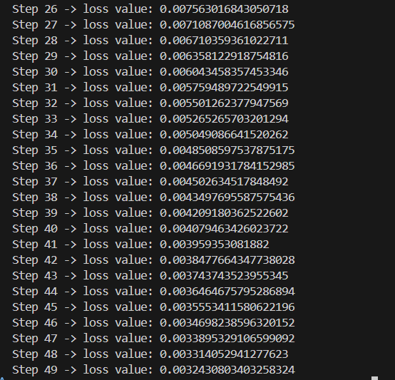
So what we did here was to overfit the model to just this batch of 50, therefore it like memorises it to the core. Now that this is done, what we actually want to do is to optimize this model as a whole. We are going to iterate the x and y values, while also create a small data loader which ensures that we keep getting fresh batches and that we are optimizing it well.
Data loader lite
class DataLoaderLite:
def __init__(self, B, T):
self.B = B
self.T = T
with open('cleaned_dataset.txt', 'r') as f:
text = f.read()
enc = tiktoken.get_encoding('gpt2')
tokens = enc.encode(text)
self.tokens = torch.tensor(tokens)
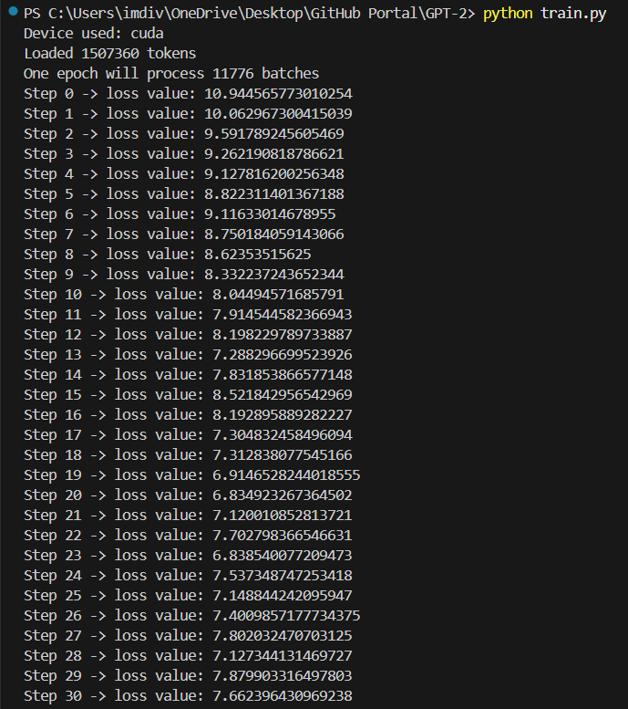
print(f"Loaded {len(self.tokens)} tokens")
print(f"One epoch will process {len(self.tokens) // (B*T)} batches")
self.current_postion = 0
def next_batch(self):
B, T = self.B, self.T
buf = self.tokens[self.current_postion : self.current_postion+B*T+1]
x = (buf[:-1]).view(B, T)
y = (buf[1:]).view(B, T)
self.current_postion += B*T
if self.current_postion + (B*T+1) > len(self.tokens):
self.current_postion = 0
return x, y
We are implementing one simple data loader here that simply goes through the file containing the data in chunks.
In the __init__ method we are reading the dataset, tokenizing it, encoding it and converting it to tensors. Finally printing how many batches get iterated in one epoch. And we set the current_position to 0.
In the next_batch method we are processing it in batches B times T. So we are loading it in batches of (B, T). So it is those chunks of batches we are processsing at the time. Therefore, even the current_position is being increated my B times T.
The buffers and setting of x, y (of setting inputs and tagets tensors) is the same as what we did in section1b dataset notebook.
Lastly, once we run out of data we just reset the current_position to 0.
train_loader = DataLoaderLite(B=4, T=32)
Here, we removed the entire '#THIS SECTION' code we saw at the start of this section and just set the DataLoader, with the same parameters.
optimizer = torch.optim.AdamW(model.parameters(), lr=3e-4)
for i in range(50):
    x, y = train_loader.next_batch()    #newly added
    x, y = x.to(device), y.to(device)   #newly added
    optimizer.zero_grad()
    logits, loss = model(x, y)
    loss.backward()
    optimizer.step()
    print(f"Step {i} -> loss value: {loss.item()}")

import sys; sys.exit(0)
Finally, we call the next_batch on x and y; and importantly move them to GPU (As by default our DataLoaderLite class processes it in CPU. Because, when we converted the input text to tokens in there, we didnt move the tokens to GPU).
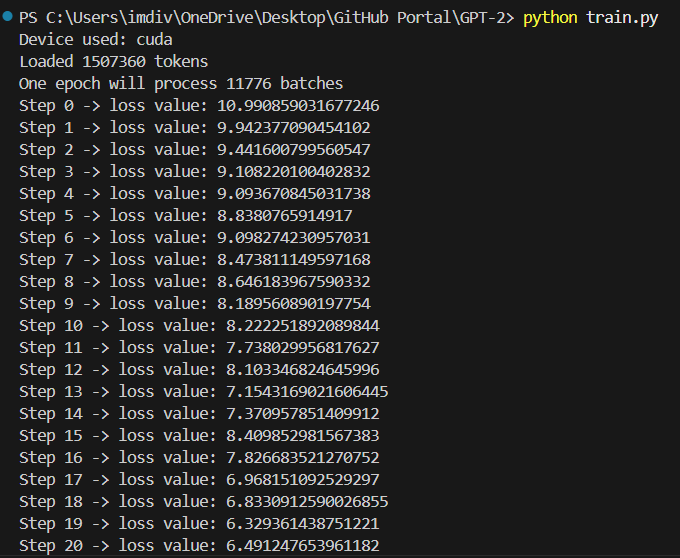
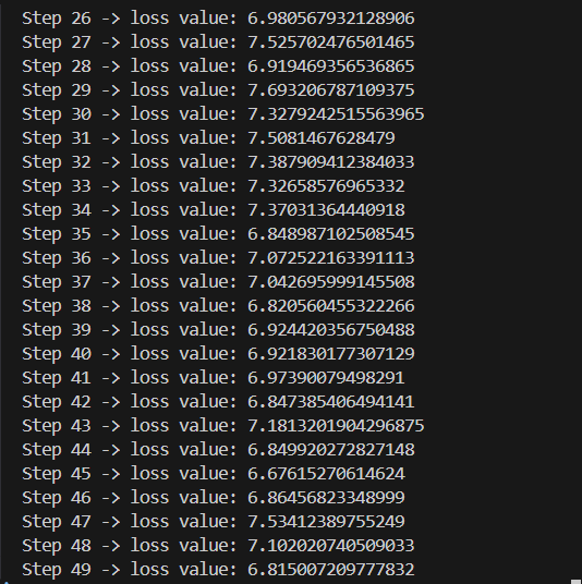
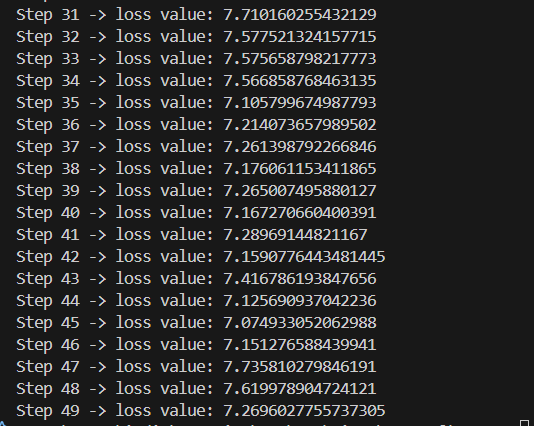
So, we ran our code to see what the loss is like now.
What's different this time, is that, just in the previous step, we only kept training on a single batch, so overfitting occured and got like a very very low loss.
This time we are adding different batches. So we expect to see a different loss value at the end. Now, although it wont be as low as before, we still expect it to be less than out estimated value, 11.
This is because, as the model learns from the data, it will notice that a lot of the tokens wont be repeated, like unicodes, special characters, complex words etc. So a lot of those will be filtered out.
But ofcourse, the ultimate aim is to get the loss close to 0, that is when our model is perfect. Since right now, we are doing only like 50 iterations, we don't expect it to go that low as seen in the output we recieved.
Parameter sharing wte and lm_head
The general idea (atleast how much i understood it)-
The tokens considered during the input and the ones produced during the output, you would expect that the tokens which have similar semantics, for example: Tokens in lower case vs in upper case, tokens with same word but in different languages; you would expect them to be near in the semantics graph. Similaryly, if it is the exact same tokens, then you would expect them to have the same weights. Therefore, at the start and end of the transformer model, there is this common property which is implemented where the similar tokens are mapped together- So, "Similar tokens should have similar properties/similar embeddings/similar weights".
Ultimately, what the researches found is that, the output embeddings are very similar to word embeddings (at the input), so they tried to tie them together and realised that they get much better outputs. This was whats done in the Attention is all you need paper and also what OpenAI did in their implementation of gpt2. Naturally, it is what we are going to implement as well :)
We only added this line of code in the end of the init method of our GPT module:
self.transformer.wte.weight = self.lm_head.weight #weight sharing scheme
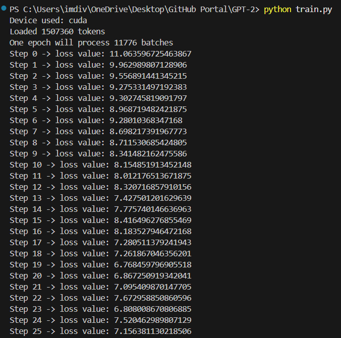
So we have implemented a weight tieing scheme and we end up saving a lot of parameters. I am still not completely sure how this effects our model, because in my case i ended up getting a higher loss value than before, but we'll see where this takes us.
Model initialization: std 0.02, residual init
Here, we are focusing on getting our initializations right as well to match with the implementation of GPT 2. There are two major updates: Initialization of standard deviation to 0.02 and Weights of the Residual layer at initialization.
Update 1:
Although the details are not mentioned explicitly, we can read between the lines in the code and find out what they have done. The notable ones would be the standard deviation to be 0.02 especially for the linear layer and token embeddings, 0.01 for positional embeddings and bias being zero. That is exactly what we will implement (except in ours, both the positional and token embeddings will be 0.02).
The custom code written by sensei:
def _init_weights(self, module):

        if isinstance(module, nn.Linear):
            torch.nn.init.normal_(module.weight, mean=0.0, std=0.02)
            if module.bias is not None:
                torch.nn.init.zeros_(module.bias)
        if isinstance(module, nn.Embedding):
            torch.nn.init.normal_(module.weight, mean=0.0, std=0.02)
funtion call at the end of init function just above:
self.apply(self._init_weights)
Apart from this, in our implementation, the only other layer that has initialization and has parameters is the Layer Norm in the MLP Module. But the PyTorch default initialization sets the scale to be 0 and offset to be 1, and that is exactly what we want.
Finally, it is important to know that, normally we would have the standard deviation as some dynamic value that would increase with the number of parameters, but here we are strictly going with what GPT 2 did, so the set value of 0.02 is added by us.
Update 2:
This is to control the growth of activations inside the residual stream in the forward pass. Now, the residual stream is as we saw during our implementation, the addition of the values as it goes up the layer and we would notice that for us those values keep on increasing. Therefore if that value is N, the paper suggests that we do a 1 to the squareroot of N. So, 1 to the square root of the number of residual layers.
So we set the following 'flag' after the c_proj in the MLP and CasualSelfAttention layers:
self.c_proj.NANOGPT_SCALE_INIT = 1
Then we add the calculation in the GPT module:
def _init_weights(self, module):

        if isinstance(module, nn.Linear):
            std = 0.02  #here
            if hasattr(module, 'NANOGPT_SCALE_INIT'):   #here
                std *= (2 * self.config.n_layer) ** -0.5    #here
            torch.nn.init.normal_(module.weight, mean=0.0, std=std)
            if module.bias is not None:
                torch.nn.init.zeros_(module.bias)
        elif isinstance(module, nn.Embedding):
            torch.nn.init.normal_(module.weight, mean=0.0, std=0.02)
The (2 * self.config.n_layer) is because we have two types of layers in a block i.e. Attention and MLP.
Here's how it performed (although i am a little concerned at this point lmao the loss is NOT getting better...?)
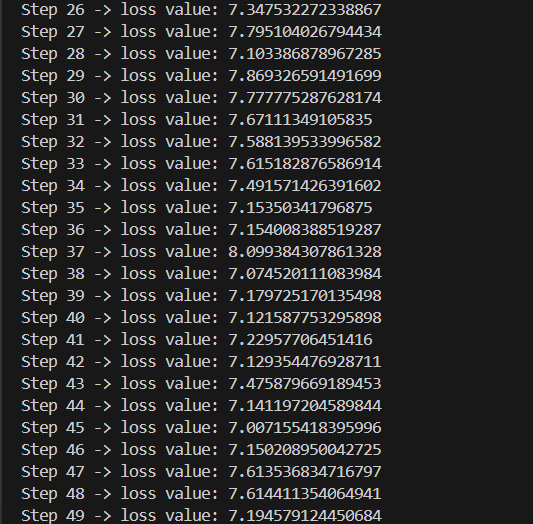
And with that, we have the initialization which is the same as in GPT 2!