
Starter Code
Importing the PyTorch and Matplotlib utilities as before
import torch
import torch.nn.functional as F
import matplotlib.pyplot as plt # for making figures
%matplotlib inline
Reading all the words
# read in all the words
words = open('names.txt', 'r').read().splitlines()
words[:8]['emma', 'olivia', 'ava', 'isabella', 'sophia', 'charlotte', 'mia', 'amelia']len(words)32033Printing the vocabulary of all the lower case letters and the special dot token
# build the vocabulary of characters and mappings to/from integers
chars = sorted(list(set(''.join(words))))
stoi = {s:i+1 for i,s in enumerate(chars)}
stoi['.'] = 0
itos = {i:s for s,i in stoi.items()}
vocab_size = len(itos)
print(itos)
print(vocab_size){1: 'a', 2: 'b', 3: 'c', 4: 'd', 5: 'e', 6: 'f', 7: 'g', 8: 'h', 9: 'i', 10: 'j', 11: 'k', 12: 'l', 13: 'm', 14: 'n', 15: 'o', 16: 'p', 17: 'q', 18: 'r', 19: 's', 20: 't', 21: 'u', 22: 'v', 23: 'w', 24: 'x', 25: 'y', 26: 'z', 0: '.'}
27Here we are reading the dataset and processing it. In the end of this cell, we are also splitting the dataset into three- Train, Dev and Loss split
# build the dataset
block_size = 3 # context length: how many characters do we take to predict the next one?

def build_dataset(words):
  X, Y = [], []

  for w in words:
    context = [0] * block_size
    for ch in w + '.':
      ix = stoi[ch]
      X.append(context)
      Y.append(ix)
      context = context[1:] + [ix] # crop and append

  X = torch.tensor(X)
  Y = torch.tensor(Y)
  print(X.shape, Y.shape)
  return X, Y

import random
random.seed(42)
random.shuffle(words)
n1 = int(0.8*len(words))
n2 = int(0.9*len(words))

Xtr,  Ytr  = build_dataset(words[:n1])     # 80%
Xdev, Ydev = build_dataset(words[n1:n2])   # 10%
Xte, Yte = build_dataset(words[n2:]) # 10%torch.Size([182625, 3]) torch.Size([182625])
torch.Size([22655, 3]) torch.Size([22655])
torch.Size([22866, 3]) torch.Size([22866])Almost the same MLP, but we have cleaned it up to add those hard coded values into variables so we just have to modify them there
# MLP revisited
n_embd = 10 # the dimensionality of the character embedding vectors
n_hidden = 200 # the number of neurons in the hidden layer of the MLP

g = torch.Generator().manual_seed(2147483647) # for reproducibility
C  = torch.randn((vocab_size, n_embd),            generator=g)
W1 = torch.randn((n_embd * block_size, n_hidden), generator=g)
b1 = torch.randn(n_hidden,                        generator=g)
W2 = torch.randn((n_hidden, vocab_size),          generator=g)
b2 = torch.randn(vocab_size,                      generator=g)

parameters = [C, W1, b1, W2, b2]
print(sum(p.nelement() for p in parameters)) # number of parameters in total
for p in parameters:
p.requires_grad = True11897Here we are optimizing the NN. Same as before, just those hard coded numbers (or magic numbers as Andrej sensei calls it) have been replaced with variable names for more readability
# same optimization as last time
max_steps = 200000
batch_size = 32
lossi = []

for i in range(max_steps):

  # minibatch construct
  ix = torch.randint(0, Xtr.shape[0], (batch_size,), generator=g)
  Xb, Yb = Xtr[ix], Ytr[ix] # batch X,Y

  # forward pass
  emb = C[Xb] # embed the characters into vectors
  embcat = emb.view(emb.shape[0], -1) # concatenate the vectors
  hpreact = embcat @ W1 + b1 # hidden layer pre-activation
  h = torch.tanh(hpreact) # hidden layer
  logits = h @ W2 + b2 # output layer
  loss = F.cross_entropy(logits, Yb) # loss function

  # backward pass
  for p in parameters:
    p.grad = None
  loss.backward()

  # update
  lr = 0.1 if i < 100000 else 0.01 # step learning rate decay
  for p in parameters:
    p.data += -lr * p.grad

  # track stats
  if i % 10000 == 0: # print every once in a while
    print(f'{i:7d}/{max_steps:7d}: {loss.item():.4f}')
lossi.append(loss.log10().item()) 0/ 200000: 27.8817
10000/ 200000: 2.8244
20000/ 200000: 2.5473
30000/ 200000: 2.8961
40000/ 200000: 2.0967
50000/ 200000: 2.5020
60000/ 200000: 2.4999
70000/ 200000: 2.0510
80000/ 200000: 2.4076
90000/ 200000: 2.3172
100000/ 200000: 2.0199
110000/ 200000: 2.3338
120000/ 200000: 1.8767
130000/ 200000: 2.3989
140000/ 200000: 2.2102
150000/ 200000: 2.1937
160000/ 200000: 2.0843
170000/ 200000: 1.8780
180000/ 200000: 1.9727
190000/ 200000: 1.8222Here we plot the loss
plt.plot(lossi)[<matplotlib.lines.Line2D at 0x28412485fc0>]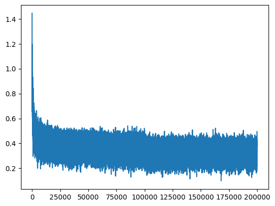
Seeing the loss in train and val loss. There is a slight modification to this as to how the splitting is done.
Here the decorator @torch.no_grad() basically tells PyTorch to not maintain the grad value, as it assumes/anticipated that the backpropagation will be calculated after this and we are saying No.
@torch.no_grad() # this decorator disables gradient tracking
def split_loss(split):
  x,y = {
    'train': (Xtr, Ytr),
    'val': (Xdev, Ydev),
    'test': (Xte, Yte),
  }[split]
  emb = C[x] # (N, block_size, n_embd)
  embcat = emb.view(emb.shape[0], -1) # concat into (N, block_size * n_embd)
  h = torch.tanh(embcat @ W1 + b1) # (N, n_hidden)
  logits = h @ W2 + b2 # (N, vocab_size)
  loss = F.cross_entropy(logits, y)
  print(split, loss.item())

split_loss('train')
split_loss('val')train 2.12243390083313
val 2.1646578311920166Sampling of the model: Forward pass -> Sampling from the distribution -> Continuing till we get the special token '.'
# sample from the model
g = torch.Generator().manual_seed(2147483647 + 10)

for _ in range(20):

    out = []
    context = [0] * block_size # initialize with all ...
    while True:
      # forward pass the neural net
      emb = C[torch.tensor([context])] # (1,block_size,d)
      h = torch.tanh(emb.view(1, -1) @ W1 + b1)
      logits = h @ W2 + b2
      probs = F.softmax(logits, dim=1)
      # sample from the distribution
      ix = torch.multinomial(probs, num_samples=1, generator=g).item()
      context = context[1:] + [ix]
      out.append(ix)
      # if we sample the special '.' token, break
      if ix == 0:
        break

print(''.join(itos[i] for i in out)) # decode and print the generated wordmora.
mayah.
see.
mel.
rylee.
emmadiejd.
leg.
adelyn.
elin.
shi.
jen.
eden.
estanar.
kayziquetta.
noshir.
roshiriel.
kendreth.
konnie.
casube.
ged.So yeah, this will be our starting point. Also use this as a revision for the previous lecture.